Deep Unsupervised Learning using Nonequilibrium Thermodynamics

2022년 현재, 생성모델로 diffusion model 인상적인 결과를 보여주며 관련 연구논문이 많이 발표되고 있다. Diffusion model쪽과 직접적으로 관련된 연구를 진행하면서 관련 연구들을 정리하는 차원에서 Diffusion model과 score-based model 논문들을 정리하고자 한다. 여기서 다루는 논문은 비교적 초기에 제시된 논문으로서 이 주제를 다루는데 있어 처음으로 읽기에 좋은 논문이라 생각되어 먼저 정리하고자 한다.
Abstract
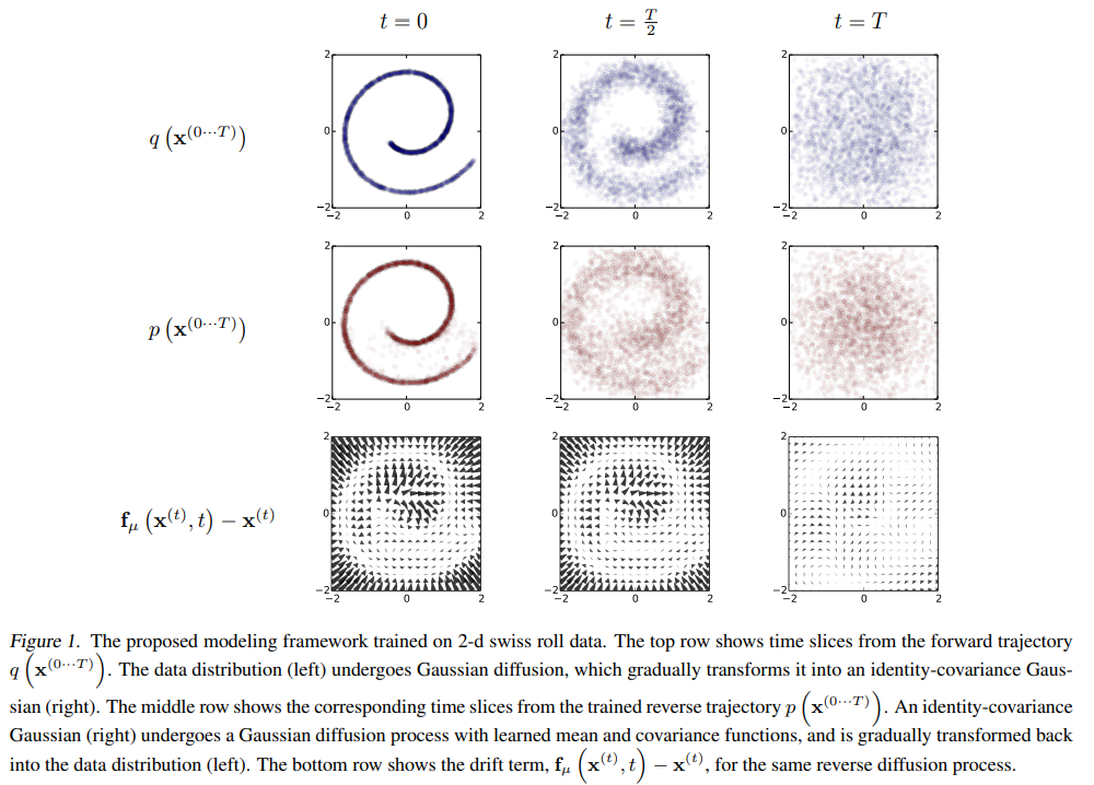
Abstract부터 상당히 흥미를 불러일으키는데, 요점은 flexible하고 동시에 tractable한 생성모델을 제시하겠다는 것이다. 그것도 non-equilibritum statistical physics라는 이름부터 상당히 어려워보이는 분야에서 영감을 받았다고 한다. 간략하게는 데이터의 분포를 단계적으로 망가뜨림으로서(diffusion process) 특정 분포를 최종적으로 만들고 이 때 각 과정의 reverse process를 학습하여 마지막 분포에서 역으로 돌아가는 과정을 만들겠다는 것이다.
Introduction
생성모델은 본질적으로 데이터가 존재할법한 분포를 파악해 “실제같은” 데이터를 만드는 것이다. 보다 범용적인 관점에서 말하면 원하는 분포(보통 이 분포가 실제 데이터들이 사는 분포겠지만)를 얼마나 잘 추정했느냐가 결과물의 품질을 결정한다고 할 수 있다. 저자는 이 과정에서 두 trade-off를 말하는데, 바로 tractability 와 flexibility이다. Tractable한 모델은 보통 확률분포를 직접 계산할 수 있는 모델을 의미한다. 예를 들어, 어떤 데이터가 주어졌을 때, 해당 데이터가 실제 분포일 확률은 얼마이다와 같이 수치적으로 계산이 가능하다. 하지만 이러한 과정은 매우, 매우 어렵다. Bayes Rule에서 posterior를 추정하는 과정에서 partitioning function이 현실적으로 계산이 불가능하다는 문제에 부딪히게 된다. 그래서 tractable하게 가기위해서는 단순한 분포, 혹은 변환을 사용해야 한다는 타협점이 생기게 된다. (예로, normalizing flow에서는 affine변환을 주로 사용한다) 반면 tractability를 포기하면 추정분포를 복잡한 분포를 사용할 수 있게되고 이렇게하면 flexibility가 올라가 고품질의 결과물을 생성하기가 수월해진다. 이러한 방법의 대표적인 접근이 GAN이다.
우선 현재로서는 diffusion process란 실제 데이터를 “어떤” 과정을 통해 여러 단계에 걸쳐 천천히 바꾸어 간단한 분포로 바꾸는 과정이라고 이해하자. 그리고 각각의 단계는 작은 변화들이기에 역과정을 추정하기가 비교적 수월할 것이며 이 역과정을 잘 학습했다면 우리는 최종적으로 도착한 간단한 분포로부터 역과정을 따라가 실제와 같은 샘플을 만들 수 있을 것임을 생각할 수 있다.
저자는 이 논문에서 diffusion probabilistic model을 제시하며 다음이 가능함을 주장한다.
- extreme flexibility in model structure, Forward process과정이 reverse process로 학습만 가능한 형태라면 분포선택에 자유도가 커지므로 보다 유연한 모델구조를 사용할 수 있다.
- exact sampling Tractability에 관한 것으로 과정이 tractable하기 때문에 정확한 분포값을 사용할 수 있다.
- easy multiplication with other distributions, e.g. in order to compute a posterior, and Posterior를 계산하기 위해서는 prior와 log-likelihood와 곱하게 되는데 1에서 언급한 이유로 다양한 분포 사용이 가능하다는 것으로 이해하였다.
- the model log likelihood, and the probability of individual states, to be cheaply evaluated log-likelihood를 직접 계산한다는 장점이 있다. 이는 실제 분포에 대해서 surrogate을 사용하지 않고 Negative log-likelihood를 loss함수에 직접 사용함으로써 목표로하는 분포에 대해 정확한 gradient를 보낼 수 있다는 강력한 장점이 있다. 다만 cheaply evaluated에 대해서는 “각각의 process에서는 적은 연산비용이겠지만 step이 수천에 이르는 diffusion process를 따른다면 전체적으로는 cheaply라고 하기에는 어려운 측면도 있지 않나?” 라는 생각이 든다.
이 방법은 Markov chain을 사용한다고 언급한다. 즉 여러 단계에 걸쳐서 다른 분포로 바꾸는 framework으로써 Markov chain을 쓰겠다는 것인데 여기서 전제되는 성질은 이름에서 알 수 있듯 Markov property이다. 즉 현재상태에서 다음상태로의 변환은 이전상태에 대해 독립적이다. 즉 transition은 이전상태와 무관하게 현재의 독립적인 사건으로 본다는 것이다. Diffusion process에서 중요한 부분은 작은 변화들을 주면서 forward process(noise형태로 만드는 과정)의 역과정을 학습하는 것이다. 따라서 각 단계의 변화가 클수록 역과정을 추론하기는 어렵다.
이 논문에서는 이러한 과정을 diffusion probabilistic model이라고 하며 toy data와 MNIST, CIFAR-10에 적용한 결과를 보여준다. 이론적인 토대는 Fokker-Planck equation에 기초하는데 이는 Kolmogorov에의해 보다 일반화된다. Kolmogorov forward and backward equation이 바로 diffusion으로 알려져 있으며 Markov process에 대한 편미분방정식(PDE)이다.
Algorithm
Diffusion process는 우선 forward diffusion을 정의하는 것에서 시작한다. 주어진 복잡한 데이터분포를 어떤 방식으로 단순하고 tractable한 분포로 바꿀지를 정해야한다. 그런 뒤에 이 과정의 역과정을 학습하면 우리는 단순한 어떤 분포로부터 데이터분포를 만드는 생성모델을 만들 수 있게 된다. 논문에서는 순서대로 forward diffusion (inference diffusion)을 정의하고 어떻게 reverse generative diffusion process를 훈련하는지를 설명한다. 그리고 어떻게 이 분포가 다른 분포와 곱해질 수 있는지를 보여준다. 다른 분포와 곱해지는 과정은 posterior를 추정하는데 필요하며 이를 통해 inpainting이나 denoising과 같은 inverse problem이 가능해진다.
Forward Trajectory
Data distributon, 즉 실제 데이터의 분포를 $q\left(\mathbf{x}^{(0)}\right)$라고 하자. 이 데이터 분포는 forward process를 통해 점차 바뀌어 결과적으로 tractable한 $\pi (\mathbf{y})$로 바뀌게 된다. 이 때 점차 바꾸어가는 과정을 Markov diffusion kernel이라고 하며 이를 $\pi(\mathbf{y})$에 대한 $T_{\pi} (\mathbf{y} \mid \mathbf{y}^{\prime} ; \beta)$라고 하며 이 때 $\beta$는 diffusion rate이다.
우선 다음의 식을 살펴보자.
$$ \begin{aligned} \pi(\mathbf{y}) &=\int d \mathbf{y}^{\prime} T_{\pi}\left(\mathbf{y} \mid \mathbf{y}^{\prime} ; \beta\right) \pi\left(\mathbf{y}^{\prime}\right) \cr q\left(\mathbf{x}^{(t)} \mid \mathbf{x}^{(t-1)}\right) &=T_{\pi}\left(\mathbf{x}^{(t)} \mid \mathbf{x}^{(t-1)} ; \beta_{t}\right) \end{aligned} $$
$\mathbf{y}^{\prime}$은 $\mathbf{y}$의 이전단계 추정이라고 생각하면, 이전단계로부터 다음단계로가는 transition을 반영하며 각각의 단계에서 $\pi (\mathbf{y}^{\prime})$은 prior처럼 역할하고 있음을 볼 수 있다. 각 변환을 총 $T$번해 최종분포로 간다고 할 때 이는 다음과 같이 써진다.
$$ q\left(\mathbf{x}^{(0 \cdots T)}\right)=q\left(\mathbf{x}^{(0)}\right) \prod_{t=1}^{T} q\left(\mathbf{x}^{(t)} \mid \mathbf{x}^{(t-1)}\right) $$
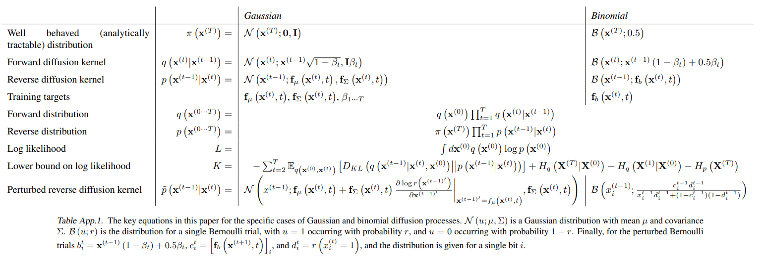
이 떄 사용된 분포 $q\left(\mathbf{x}^{(t)} \mid \mathbf{x}^{(t-1)}\right)$는 본 논문에서 Gaussian과 binomial distribution이 사용되었다. 실제 분포에 대한 식은 아래의 appendix table에 정리가 잘 되어있다.
Reverse Trajectory
Forward diffusion process는 명료하다. 분포를 정하고 그 분포에 따라 변환시키는 것이다. 여기서는 이 역과정을 추정하는 방법을 다룬다. 이는 생성과정이기 때문에 generative distribution이라고 하며 다음과 같이 쓸 수 있다.
$$ \begin{aligned} p\left(\mathbf{x}^{(T)}\right) &=\pi\left(\mathbf{x}^{(T)}\right) \cr p\left(\mathbf{x}^{(0 \cdots T)}\right) &=p\left(\mathbf{x}^{(T)}\right) \prod_{t=1}^{T} p\left(\mathbf{x}^{(t-1)} \mid \mathbf{x}^{(t)}\right) \end{aligned} $$
Binomial이나 Gaussian의 경우는 step size $\beta$가 매우 작다면 reverse diffusion process가 forward와 같음이 알려져있다.(Feller, 1949) 따라서 $q\left( \mathbf{x}^{(t)} \mid \mathbf{x}^{(t-1)} \right)$가 Gaussian이라면 $\beta_t$가 작을 때, $q\left( \mathbf{x}^{(t-1)} \mid \mathbf{x}^{(t)} \right)$도 Gaussian이 된다. Trajectory를 길게 만들수록 $beta_t$를 작게 만들 수 있으므로 위의 명제의 “$\beta$가 매우 작다면"이라는 가정을 더 만족시킬 수 있게 된다. 그렇다면 reverse에서 Gaussian의 경우를 추정한다고 해보자. Gaussian은 mean과 variance만으로 정의할 수 있다는 장점이 있다. 즉 mean과 variance를 추정해야하며 이는 Table App.1.에서 $\mathbf{f}_{\mu} (\mathbf{x}^{(t)}, t)$, $\mathbf{f}_{\Sigma} (\mathbf{x}^{(t)}, t)$로 표현되어있다. 이 떄 $t$에 conditioning 되어 있음에 유의하자. 즉 process 각각에 대해 conditioning이 될 것임을 짐작할 수 있다.
Diffusion process에서의 계산비용은 따라서 위의 reverse diffusion process과정에 대한 학습을 time-step만큼 곱한만큼이 된다. 여기서 평균과 분산을 추정하는 함수로는 간단한 MLP가 사용되었다.
Model Probability
Diffusion process에 따라 생성모델이 데이터에 부여하는 확률은 다음과 같다.
$$ p\left(\mathbf{x}^{(0)}\right)=\int d \mathbf{x}^{(1 \cdots T)} p\left(\mathbf{x}^{(0 \cdots T)}\right) $$
위의 식은 intractable하다. 각 sample과 $p$의 모든 time-step을 고려할 수 없다. 하지만 저자는 annealed importance sampling과 Jarzynski equality를 사용해 다음처럼 전개할 수 있다고 한다.
$$ \begin{aligned} p\left(\mathbf{x}^{(0)}\right) &=\int d \mathbf{x}^{(1 \cdots T)} p\left(\mathbf{x}^{(0 \cdots T)}\right) \frac{q\left(\mathbf{x}^{(1 \cdots T)} \mid \mathbf{x}^{(0)}\right)}{q\left(\mathbf{x}^{(1 \cdots T)} \mid \mathbf{x}^{(0)}\right)} \cr &=\int d \mathbf{x}^{(1 \cdots T)} q\left(\mathbf{x}^{(1 \cdots T)} \mid \mathbf{x}^{(0)}\right) \frac{p\left(\mathbf{x}^{(0 \cdots T)}\right)}{q\left(\mathbf{x}^{(1 \cdots T)} \mid \mathbf{x}^{(0)}\right)} \cr &=\int d \mathbf{x}^{(1 \cdots T)} q\left(\mathbf{x}^{(1 \cdots T)} \mid \mathbf{x}^{(0)}\right) \cr & p\left(\mathbf{x}^{(T)}\right) \prod_{t=1}^{T} \frac{p\left(\mathbf{x}^{(t-1)} \mid \mathbf{x}^{(t)}\right)}{q\left(\mathbf{x}^{(t)} \mid \mathbf{x}^{(t-1)}\right)} \end{aligned} $$
위에서 마지막식으로 가는 과정이 tractable해지기 위한 핵심적인 과정이라고 생각하며 이 때 ancestral sampling으로 intractable한 상황을 비켜갔음을 볼 수 있다. 그리고 $\beta$가 매우 작다면 forward와 reverse 분포가 같아지므로 이 경우에는 $q\left(\mathbf{x}^{(1 \cdots T)} \mid \mathbf{x}^{(0)}\right)$만으로 적분을 할 수 있다. 바로 이 부분이 통계물리의 quasi-static process에 해당한다고 저자는 이야기한다.
Training
Normalizing flow가 그러했듯 tractable한 분포를 설계함으로 인해 얻는 큰 장점중 하나는 바로 likelihood를 최대화하는 방식으로 objective를 정할 수 있다는 것이다.
$$ \begin{aligned} L &=\int d \mathbf{x}^{(0)} q\left(\mathbf{x}^{(0)}\right) \log p\left(\mathbf{x}^{(0)}\right) \cr &=\int d \mathbf{x}^{(0)} q\left(\mathbf{x}^{(0)}\right) \cdot \cr & \log \left[\begin{array}{r} \int d \mathbf{x}^{(1 \cdots T)} q\left(\mathbf{x}^{(1 \cdots T)} \mid \mathbf{x}^{(0)}\right) \cr p\left(\mathbf{x}^{(T)}\right) \prod_{t=1}^{T} \frac{p\left(\mathbf{x}^{(t-1)} \mid \mathbf{x}^{(t)}\right)}{q\left(\mathbf{x}^{(t)} \mid \mathbf{x}^{(t-1)}\right)}\end{array}\right] \end{aligned} $$
Jansen’s inequality에 의해 다음과 같은 lower bound를 갖게 된다.
$$ \begin{aligned} &L \geq \int d \mathbf{x}^{(0 \cdots T)} q\left(\mathbf{x}^{(0 \cdots T)}\right) \cr &\log \left[p\left(\mathbf{x}^{(T)}\right) \prod_{t=1}^{T} \frac{p\left(\mathbf{x}^{(t-1)} \mid \mathbf{x}^{(t)}\right)}{q\left(\mathbf{x}^{(t)} \mid \mathbf{x}^{(t-1)}\right)}\right] \end{aligned} $$
Appendix B에서 위는 다음으로 유도된다.
$$ \begin{aligned} L & \geq K \cr K=&-\sum_{t=2}^{T} \int d \mathbf{x}^{(0)} d \mathbf{x}^{(t)} q\left(\mathbf{x}^{(0)}, \mathbf{x}^{(t)}\right) \cr & D_{K L}\left(q\left(\mathbf{x}^{(t-1)} \mid \mathbf{x}^{(t)}, \mathbf{x}^{(0)}\right)|| p\left(\mathbf{x}^{(t-1)} \mid \mathbf{x}^{(t)}\right)\right) \cr &+H_{q}\left(\mathbf{X}^{(T)} \mid \mathbf{X}^{(0)}\right)-H_{q}\left(\mathbf{X}^{(1)} \mid \mathbf{X}^{(0)}\right)-H_{p}\left(\mathbf{X}^{(T)}\right) \end{aligned} $$
이때 entropy와 KL divergence는 계산이 가능하므로 위 식은 계산할 수 있다. 재미있는점은 여기서 lower bound를 계산하였으므로 더이상 엄밀한 log-likelihood를 계산하는 것이 아닌 surrogate objective를 사용하게 되었다는 점이다. 물론 게산가능해야 무엇인든 해볼 수 있으므로 어쩔 수 없는 타협이라고 생각한다. 하지만 위 식에서 equality가 성립하는 경우가 바로 forward와 reverse가 동일할 때이다. 즉 이 타협은 $\beta_t$를 충분히 작게함으로써 완화될 수 있는 부분이라고 생각한다.
Reverse Markov transition은 이제 다음에 대한 surrogate $K$를 maximize하는 문제로 바뀌었다.
$$ \hat{p}\left(\mathbf{x}^{(t-1)} \mid \mathbf{x}^{(t)}\right)=\underset{p\left(\mathbf{x}^{(t-1)} \mid \mathbf{x}^{(t)}\right)}{\operatorname{argmax}} K $$
이러한 과정을 거치는 이유는 reverse process를 추정하기위한 것으로 결국 Gaussian forward process였다면 reverse process의 평균과 분산을 추정하는 문제로 단순화시키기 위함이다.
Setting the Diffusion Rate $\beta_t$
앞서 과정들에서 언급이 되었듯 $\beta_t$를 정하는 것은 성능에 매우 중요했다고 한다. Gaussian diffusion 과정에서 diffusion schedule을 K에 대한 gradient ascent로 학습하였다고 한다. 다만, 분산의 $\beta_1$, 즉 첫번째 step에 대해서는 overfitting을 막기 위해 학습하지 않고 작은 constant를 사용하였다고한다.
Multiplying Distributions, and Computing Posteriors
Denoising이나 inpainting과 같은 작업을 하기 위해서는 model distributino에 다른 분포가 곱해지는 형태로 다음과 같은 분포를 사용해 풀 수 있다.
$$ \tilde{p}\left(\mathbf{x}^{(0)}\right) \propto p\left(\mathbf{x}^{(0)}\right) r\left(\mathbf{x}^{(0)}\right) $$
분포를 곱하는 것은 쉬운일이 아니다. 하지만 Diffusion model에서는 곱하는 분포를 diffusion process에서 perturbation으로 간주하여 단순화할 수 있다.
Modified Marginal Distribution
위의 $\tilde{p}$를 계산하기 위해서는 각각의 reverse process에 $r(\mathbf{x}^{(t)})$가 곱해져야 한다. $\tilde{p}$도 확률의 성질을 만족해야하므로 normalizing constant를 계산해 다음과 같이 정의되어야 한다.
$$ \tilde{p}\left(\mathbf{x}^{(t)}\right)=\frac{1}{\tilde{Z}_{t}} p\left(\mathbf{x}^{(t)}\right) r\left(\mathbf{x}^{(t)}\right) $$
Marov kernel $p(\mathbf{x}^{(t) \mid \mathbf{x}^(t+1)})$은 다음의 equilibrium condition을 따라야 한다.
$$ p\left(\mathbf{x}^{(t)}\right)=\int d \mathbf{x}^{(t+1)} p\left(\mathbf{x}^{t)} \mid \mathbf{x}^{(t+1)}\right) p\left(\mathbf{x}^{t+1)}\right) $$
Perturbed markov에 대해서도 동일하게 적용하면 다음과 같다.
$$ \begin{aligned} \tilde{p}\left(\mathbf{x}^{(t)}\right) &= \int d \mathbf{x}^{(t+1)} \tilde{p}\left(\mathbf{x}^{(t)} \mid \mathbf{x}^{(t+1)}\right) \tilde{p}\left(\mathbf{x}^{t+1)}\right)\cr \frac{p\left(\mathbf{x}^{(t)}\right) r\left(\mathbf{x}^{(t)}\right)}{\tilde{Z}_{t}} &=\int d \mathbf{x}^{(t+1)} \tilde{p}\left(\mathbf{x}^{(t)} \mid \mathbf{x}^{(t+1)}\right) \frac{p\left(\mathbf{x}^{(t+1)}\right) r\left(\mathbf{x}^{(t+1)}\right)}{\tilde{Z}_{t+1}} \cr p\left(\mathbf{x}^{(t)}\right) &=\int d \mathbf{x}^{(t+1)} \tilde{p}\left(\mathbf{x}^{(t)} \mid \mathbf{x}^{(t+1)}\right) \frac{\tilde{Z}_{t} r\left(\mathbf{x}^{(t+1)}\right)}{\tilde{Z}_{t+1} r\left(\mathbf{x}^{(t)}\right)} p\left(\mathbf{x}^{(t+1)}\right) \end{aligned} $$
다음이 만족되면 위의 마지막식은 기존 유도와 같은 형태가 됨을 알 수 있다.
$$ \tilde{p}\left(\mathbf{x}^{(t)} \mid \mathbf{x}^{(t+1)}\right)=p\left(\mathbf{x}^{(t)} \mid \mathbf{x}^{(t+1)}\right) \frac{\tilde{Z}_{t+1} r\left(\mathbf{x}^{(t)}\right)}{\tilde{Z}_{t} r\left(\mathbf{x}^{(t+1)}\right)} \tag{21} $$
다만 위 식은 normalized probability distribution이 된다는 보장이 없다. 따라서 이를 확률분포로 만들기 위해 다음처럼 $\tilde{p} \left( \mathbf{x}^{(t)} \mid \mathbf{x}^{(t+1)}\right)$을 정의한다.
$$ \tilde{p}\left(\mathbf{x}^{(t)} \mid \mathbf{x}^{(t+1)}\right)=\frac{1}{\tilde{Z}_{t}\left(\mathbf{x}^{(t+1)}\right)} p\left(\mathbf{x}^{(t)} \mid \mathbf{x}^{(t+1)}\right) r\left(\mathbf{x}^{(t)}\right) \tag{22} $$ 이 때, $\tilde{Z}_{t} \elft \mathbf{x}^{(t+1)} \right)$는 normalization constant이다.
Gaussian에 대해서는 각각의 step에서 $r\left(\mathbf{x}^{(t)}\rigiht)$에서 매우 급격하게 큰 값을 갖는다고 한다. 기존에는 small perturbation으로 움직이는데 어떤 positive function $r$이 개입되면서 분포에 영향을 많이 준 것으로 이해하였다. 다만 저자는 $\frac{r\left(\mathbf{x}^{(t)}\right)}{r\left(\mathbf{x}^{(t+1)}\right)}$는 $p(\mathbf{x}^{(t)} \mid \mathbf{x}^{(t+1)})$에 대한 small perturbation으로 볼 수 있음을 말한다. 따라서 위의 (21)을 보면 Gaussian에 대한 작은 perturbation이로 볼 수있고 21과 22는 Appendix C에 의해 같아지게 된다.
Applying $r\left(\mathbf{x}^{(t)}\right)$
만약 $r\left(\mathbf{x}^{(t)}\right)$가 충분히 부드럽다면 이는 reverse diffusion kernel에 대해 small perturbation으로 여겨질 수 있고 이 때 $\tilde{p}$는 $p$와 같은 형태를 갖는다.
Choosing $r\left(\mathbf{x}^{(t)}\right)$
그렇다면 $r\left(\mathbf{x}^{(t)}\right)$는 어떻게 골라야 하는지를 알아보자. $r\left(\mathbf{x}^{(t)}\right)$는 trajectory에 따라 천천히 변할 수 있는 함수로 골라야한다. 논문에서는 상수로 정했다고 한다.
$$ r\left(\mathbf{x}^{(t)}\right)=r\left(\mathbf{x}^{(0)}\right) $$
$r\left(\mathbf{x}^{(t)}\right)=r\left(\mathbf{x}^{(0)}\right)^{\frac{T-t}{T}}$로 정하는 방법도 있는데 이렇게하면 $r$은 reverse trajectory의 시작분포에 대해 contribution이 없으므로 ($t=T$), $\tilde{p}$에서 최초 sample을 뽑는과정이 기존과 동일해지게 된다.
Entropy of Reverse Process
Forward process는 알고 있으므로 reverse trajectory에서의 각 단계에서의 conditional entropy의 upper & lower bound를 유도할 수 있다.
$$ \begin{array}{r} H_{q}\left(\mathbf{X}^{(t)} \mid \mathbf{X}^{(t-1)}\right)+H_{q}\left(\mathbf{X}^{(t-1)} \mid \mathbf{X}^{(0)}\right)-H_{q}\left(\mathbf{X}^{(t)} \mid \mathbf{X}^{(0)}\right) \cr \leq H_{q}\left(\mathbf{X}^{(t-1)} \mid \mathbf{X}^{(t)}\right) \leq H_{q}\left(\mathbf{X}^{(t)} \mid \mathbf{X}^{(t-1)}\right) \end{array} $$ 이 때 upper, lower bound는 모두 $q(\mathbf{x}^(1 \cdots T) \mid \mathbf{x}^{(0)})$에 의존하며 analytic하게 계산될 수 있다. (Appendix A에서 유도된다)
Experiments
실험에서는 toy data와 MNIST, CIFAR10, Dead Leaf Images 데이터 셋에 대해서 생성 및 inpainting을 보여준다. 각각의 결과물을 볼 때, 생성능력자체가 엄청나게 뛰어나지는 않지만 diffusion process로서 이러한 작업을 할 수 있음을 보여주었다는데 의의가 있다.
Bibliography
Sohl-Dickstein, Jascha, et al. “Deep unsupervised learning using nonequilibrium thermodynamics.” International Conference on Machine Learning. PMLR, 2015.