Score-based Generative Model

Generative models are a class of machine learning models that learn to create data resembling the distribution of their training set. In essence, they can produce “realistic” data that could plausibly exist in the real world. Over the years, researchers have proposed various frameworks to achieve this goal, including GANs (Generative Adversarial Networks), VAEs (Variational Autoencoders), and Normalizing Flows. Each of these approaches continues to evolve, aiming to generate increasingly natural and realistic data.

This blog post draws inspiration from the paper “Generative Modeling by Estimating Gradients of the Data Distribution,” with Yang Song as the first author. However, rather than providing a formal paper review, we’ll focus on understanding generative models in general while exploring the background and key concepts of the score-based generative model presented in the paper.

This post is primarily based on a seminar by Professor Stefano Ermon, which offers valuable insights.

Benefits of Accessing Probability Mass/Density Function

Let’s first look at the classification system used by Ian Goodfellow in his NIPS 2016 Tutorial presentation “NIPS 2016 Tutorial: Generative Adversarial Networks”.

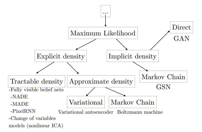
GANs are classified as having implicit density. Considering the structure of GANs, they start with random noise and generate samples by passing through the GAN generator. As we’ll emphasize later, when modeling probabilities, it’s crucial to satisfy the basic properties of probability: the sum must be 1, and it can never be negative anywhere. However, given the size of the probability space we’re dealing with, making the sum equal to 1 is no easy task. The function that normalizes it to 1 is called the partition function, and finding this function itself is challenging. While it would be great to directly increase the likelihood of this probability if we could define the probability distribution, this process is ultimately difficult. GANs were able to avoid the challenge of directly modeling the probability distribution by adversarially training a generative model and a discriminative model (a two-player minimax game). This can be confirmed by the fact that likelihood is not used anywhere in the GAN training process. While successful in generating results, the downside is that, aside from the difficulties in training, there are limitations in using the probability distribution because the estimation of the probability distribution is not explicitly revealed during the training process.

VAEs, although unable to directly optimize probabilities, can estimate probability distributions indirectly by deriving and optimizing the evidence lower bound, making it a framework that can approach probability distributions more closely than GANs. Of course, there were issues such as forced use of Gaussian priors and lower quality of final results compared to what GANs produce, but these drawbacks are being rapidly improved with the emergence of methods like VQ-VAE.

Normalizing flows model probability distributions through tractable layers, with the most powerful advantage being that they can directly optimize the log-likelihood of the probability distribution as they estimate the probability distribution tractably. However, to ensure tractability, they must be invertible, and the determinant of the transformation applied at each step must be easily calculable.

The core issue here is that “it’s difficult to directly access the probability distribution.” If we could directly access the probability mass/density function, it would be the distribution of the data we want to find, so we could optimize to be close to this distribution. However, because it must satisfy the properties of probability distributions, it’s difficult to formulate in the modeling process, making it challenging to use the maximum likelihood approach. The trade-off is that if we assume a simple probability distribution, it becomes tractable and directly optimizable, but assuming a simple probability distribution greatly limits the expressivity of the data and makes it impossible to model complex forms of data.

Score

In his paper, Yang Song proposes a novel framework that differs from existing approaches. This new method is called score-based generative modeling. Let’s explore it step by step.

First, we need to understand what “score” means in this context. In the realm of generative models, the score is defined as follows:

The score is the gradient of the log of the data’s probability distribution.

\[\nabla_x \log p(\mathbf{x})\]

It’s important to note that this score is the gradient with respect to the input data, not the model parameters.

Let’s consider a probability distribution composed of two Gaussian mixtures with means at \((-1.5, 1.5)\) and \((1.0, 1.0)\).

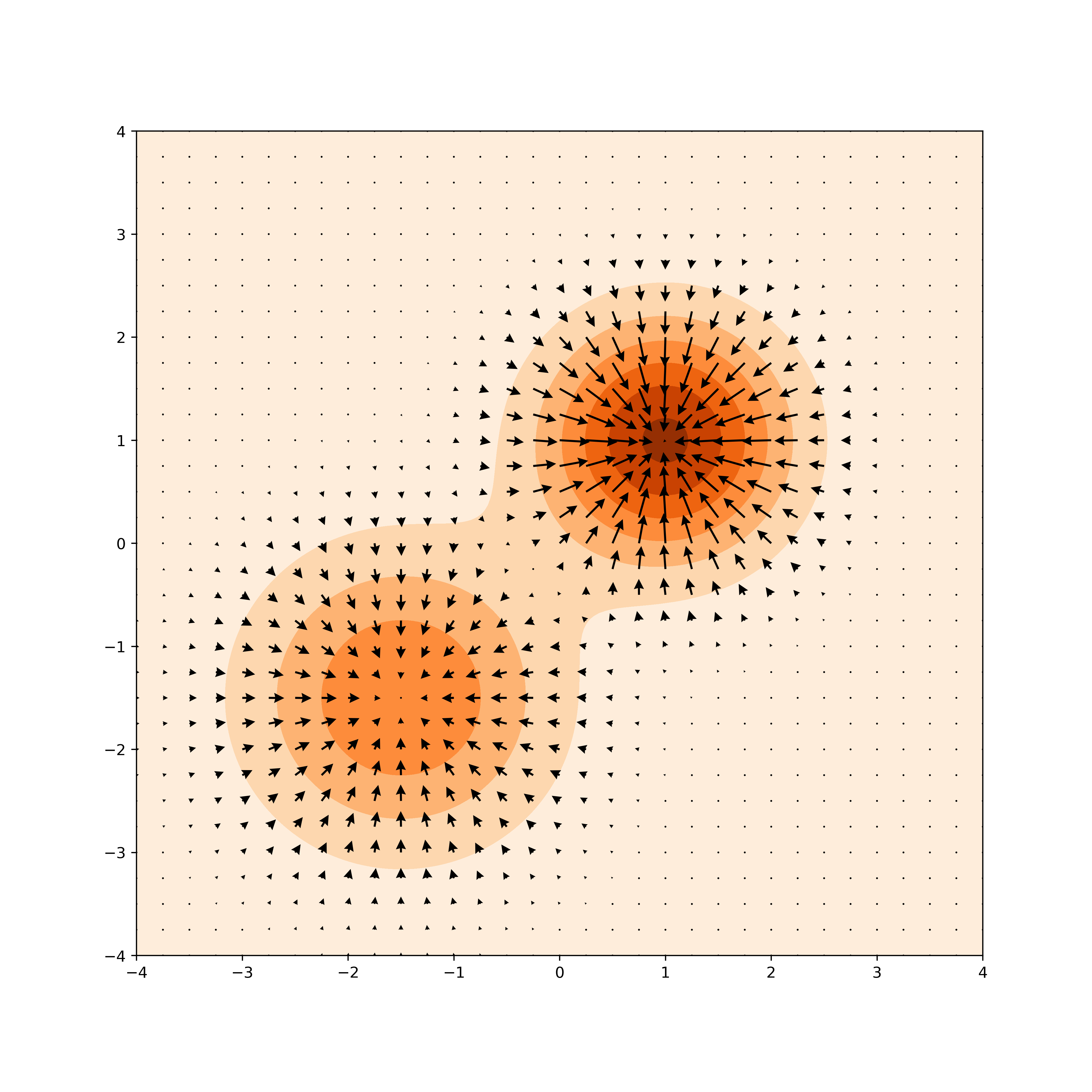
In this image, the score is represented as a vector field of gradients, visualized by arrows. The score indicates how to move from any given point to reach areas of higher likelihood. Following these arrows in our distribution would lead to the mean vectors of each Gaussian.

The core idea of score-based models is to utilize this score directly instead of working with the probability distribution function itself.

Deep Energy-Based Models

The concept of using scores in models is not new. Energy-based models aim to create a network that outputs an arbitrary real number for an input \(\mathbf{x}\), and then use this value to estimate a probability distribution using the following equation:

\[f_{\theta}(\mathbf{x}) \in \mathbb{R}\] \[p_{\theta}(\mathbf{x}) = \frac{e^{-f_{\theta}(\mathbf{x})}}{Z_{\theta}}\]

The network outputs an arbitrary real number \(f_{\theta}(\mathbf{x})\), which can be negative. By applying the exponential function, we can ensure the output is positive, addressing the condition that probabilities must be non-negative. However, the main challenge lies in ensuring that the sum of the probability distribution equals 1. This is represented by the normalization constant \(Z_{\theta}\) (Normalizing Constant or Partition Function), which is the sum of the exponential values of all possible inputs, which is often intractable to compute.

To train such a model using log-likelihood, we need to calculate the following Negative Log-Likelihood (NLL) loss:

\[\mathbb{E}_{p_{\text{data}}}[-\log p_{\theta}(\mathbf{x})] = \mathbb{E}_{p_{\text{data}}}[f_{\theta}(\mathbf{x}) + \log Z_{\theta}]\]

The intractability of \(Z_{\theta}\) makes it impossible to use Maximum Likelihood Estimation (MLE) directly for training these models.

This intractability issue is a significant challenge in energy-based models and has led to the development of various approximation techniques and alternative training methods in the field of deep learning and probabilistic modeling.

Learning Deep Energy-Based Models using Scores

In the context of energy-based models, the score function plays a crucial role in simplifying the learning process. The score is defined as the gradient of the log-probability with respect to the input. One of the key advantages of working with scores is that they are independent of the partition function, which often poses computational challenges in energy-based models.

Consider the following equation:

\[\nabla_{\mathbf{x}} \log p_{\theta}(\mathbf{x}) = - \nabla_{\mathbf{x}} f_{\theta}(x) - \nabla_{\mathbf{x}} \log Z_{\theta}\]

Where:

• \(p_{\theta}(\mathbf{x})\) is the probability distribution
• \(f_{\theta}(x)\) is the energy function
• \(Z_{\theta}\) is the partition function

The insight here is that we can treat the gradient of the partition function with respect to \(\mathbf{x}\) as zero. This simplification is possible because the score doesn’t affect the partition function.

The partition function \(Z_{\theta}\) is defined as:

\[Z_{\theta} = \int e^{-f_{\theta}(\mathbf{x})} \mathrm{d} \mathbf{x}\]

The partition function is defined as the sum of the exponential values of all possible inputs. The integral sums up the exponential of the negative energy for every possible input \(\mathbf{x}\) in the input space. It is not evaluating the function at a specific point but rather integrating over the entire input space. Note that \(\theta\) represents the parameters of the model. If we change the parameters, the entire function \(f_{\theta}(\mathbf{x})\) changes, leading to a different partition function. On the other hand, \(\mathbf{x}\) represents the input data. It is not a fixed value but ranges over all possible inputs.

This leads to a fundamental idea: while working directly with probability distributions requires dealing with the challenging partition function, estimating the score can be done without involving the partition function at all.

Let’s denote the score function of the real data distribution as \(\nabla_{\mathbf{x}} \log p_{\text{data}}(\mathbf{x})\). The core concept is to train a neural network with parameters \(\theta\) so that its score function \(\nabla_{\mathbf{x}} \log p_{\theta}(\mathbf{x})\) approximates the true data score \(\nabla_{\mathbf{x}} \log p_{\text{data}}(\mathbf{x})\).

Score Estimation

Let’s clarify the problem setting. Our goal is to estimate the data distribution \(p_{\text{data}}(\mathbf{x})\), which we can’t calculate directly due to the partition function. Instead, we approach this through the score function.

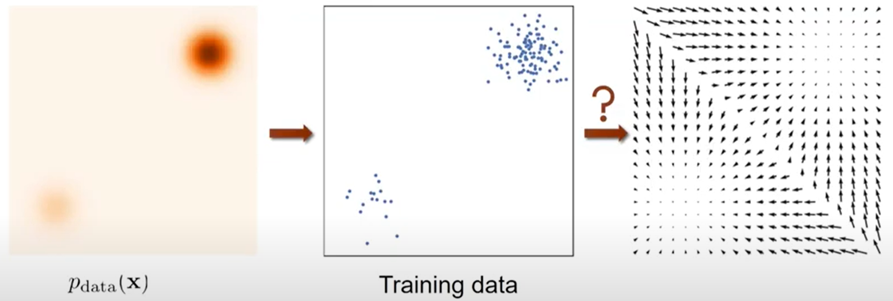
As shown in the image above, we don’t know the actual distribution. We only have access to training data sampled from this distribution. Our task is to estimate the score function of this training data. However, the training data itself doesn’t contain information about gradients. This brings us to a more specific problem: How can we estimate a score function \(s_{\theta}(\mathbf{x}): \mathbb{R}^D \rightarrow \mathbb{R}^{D}\) that approximates \(\nabla_{\mathbf{x}} \log p_{\text{data}}(\mathbf{x})\) using only the training data? In essence, we need to find the vector field that represents the scores of the actual data. Here, \(D\) represents the dimension of the data.

Let’s formulate the problem more precisely:

• Given: i.i.d. samples \(\{ \mathbf{x}_1, \mathbf{x}_2, \cdots, \mathbf{x}_{N} \} \stackrel{\text{i.i.d.}}{\sim} p_{\text{data}} (\mathbf{x}) = p(\mathbf{x})\)
• Task: Estimate the score \(\nabla_{\mathbf{x}} \log p(\mathbf{x})\)
• Score Model: A vector-valued function \(s_{\theta}(\mathbf{x}): \mathbb{R}^{D} \rightarrow \mathbb{R}^{D}\)
• Objective: Determine how to compare two vector fields of scores

This formulation presents several challenges:

1. We’re working with high-dimensional data (represented by \(D\)).
2. We need to design a model \(s_{\theta}\) that can effectively capture the complex relationships in the data.
3. We need to develop a method to train this model using only the samples, without direct access to the true score.

Score Matching

The goal is to make a parameterized function \(s_{\theta}\) equal to \(\nabla_{\mathbf{x}} \log p(\mathbf{x})\). If we define the distance using Euclidean distance, we can set up the following loss function:

\[\frac{1}{2} \mathbb{E}_{p(\mathbf{x})} \left[ \lVert \nabla_{\mathbf{x}} \log p(\mathbf{x}) - s_{\theta}(\mathbf{x}) \rVert_2^2 \right]\]

The left side represents the true score, while the right side is the network trying to estimate it. This expression is called the Fisher divergence. When the Fisher divergence is 0, the two distributions are identical.

However, we still face a problem: we don’t know \(p(\mathbf{x})\), so we can’t calculate its score, making it impossible to compute the true score term on the left. By using integration by parts, we can transform the above expression into:

\[\mathbb{E}_{p(\mathbf{x})}\left[\frac{1}{2} \lVert s_{\theta}(\mathbf{x}) \rVert_{2}^{2}+\operatorname{tr}(\underbrace{\nabla_{\mathbf{x}} s_{\theta}(\mathbf{x})}_{\text {Jacobian of } s_{\theta}(\mathbf{x})})\right]\]

The advantage of this transformation is that we can eliminate \(p(\mathbf{x})\) from the equation. This process is called Score Matching (Hyvarinen, 2005). Now, \(p(\mathbf{x})\) only remains in the expectation, allowing us to estimate it using training data as follows:

\[\frac{1}{N} \sum_{i=1}^{N}\left[\frac{1}{2} \lVert s_{\theta}\left(\mathbf{x}_{i}\right) \rVert_{2}^{2}+\operatorname{tr}\left(\nabla_{\mathbf{x}} s_{\theta}\left(\mathbf{x}_{i}\right)\right)\right], \quad \{ \mathbf{x}_{1}, \mathbf{x}_{2}, \ldots, \mathbf{x}_{N} \} \stackrel{\text{i.i.d.}}{\sim} p(\mathbf{x})\]

Derivation

To understand the score matching process mentioned above, let’s examine an example using one-dimensional data.

\[\begin{aligned} & \frac{1}{2} \mathbb{E}_{p(x)}\left[\left(\nabla_{x} \log p(x)-s_{\theta}(x)\right)^{2}\right] \cr =& \frac{1}{2} \int p(x)\left(\nabla_{x} \log p(x)-s_{\theta}(x)\right)^{2} \mathrm{~d} x \cr =& \frac{1}{2} \int p(x)\left(\nabla_{x} \log p(x)\right)^{2} \mathrm{~d} x+\frac{1}{2} \int p(x) s_{\theta}(x)^{2} \mathrm{~d} x \cr &-\int p(x) \nabla_{x} \log p(x) s_{\theta}(x) \mathrm{d} x \end{aligned}\]

In this expansion, the first term is independent of \(\theta\). The second term can be easily wrapped in an expectation. The last term is problematic, but it can be rewritten as follows:

\[\begin{aligned} &-\int p(x) \nabla_{x} \log p(x) s_{\theta}(x) \mathrm{d} x \cr =&-\int p(x) \frac{\nabla_{x} p(x)}{p(x)} s_{\theta}(x) \mathrm{d} x=-\int \nabla_{x} p(x) s_{\theta}(x) \mathrm{d} x \cr =&-\left.p(x) s_{\theta}(x)\right|_{x=-\infty} ^{\infty}+\int p(x) \nabla_{x} s_{\theta}(x) \mathrm{d} x \cr =& \int p(x) \nabla_{x} s_{\theta}(x) \mathrm{d} x \end{aligned}\]

The boundary term in the third line will be zero for \(\pm \infty\), so the result can be expressed as an expectation.

For a one-dimensional \(D\), we can rewrite it as follows:

\[\begin{aligned} & \frac{1}{2} \mathbb{E}_{p(x)}\left[\left(\nabla_{x} \log p(x)-s_{\theta}(x)\right)^{2}\right] \cr =& \frac{1}{2} \int p(x)\left(\nabla_{x} \log p(x)\right)^{2} \mathrm{~d} x+\frac{1}{2} \int p(x) s_{\theta}(x)^{2} \mathrm{~d} x \cr &+\int p(x) \nabla_{x} s_{\theta}(x) \mathrm{d} x \cr =& \text{const} +\frac{1}{2} \mathbb{E}_{p(x)}\left[s_{\theta}(x)^{2}\right]+\mathbb{E}_{p(x)}\left[\nabla_{x} s_{\theta}(x)\right] \end{aligned}\]

Using the same principle, for \(D \geq 1\), it can be derived as shown above.

Why Score Matching is Not Scalable

Score matching is a powerful technique that allows us to find the score function by reducing the cost function through Monte Carlo methods. This, in turn, enables us to train a network to estimate the true score we’re interested in. However, a significant problem remains: score matching is not scalable. Let’s examine this issue in detail.

Imagine we have data represented by three variables. In this case, our input data \(\mathbf{x}\) belongs to \(\mathbb{R}^3\), and the score function \(s_{\theta}(\mathbf{x})\) is a function from \(\mathbb{R}^{D}\) to \(\mathbb{R}^{D}\), also producing three output values.

The cost function for score matching is given by:

\[\mathbb{E}_{p(\mathbf{x})}\left[\frac{1}{2} \lVert s_{\theta}(\mathbf{x}) \rVert_{2}^{2}+\operatorname{tr}(\underbrace{\nabla_{\mathbf{x}} s_{\theta}(\mathbf{x})}_{\text {Jacobian of } s_{\theta}(\mathbf{x})})\right]\]

To compute this, we need to calculate two terms: \(\lVert s_{\theta} (\mathbf{x}) \rVert_2^2\) and \(\operatorname{tr}(\nabla_{\mathbf{x}} s_{\theta}(\mathbf{x}))\). While calculating \(\lVert s_{\theta} (\mathbf{x}) \rVert_2^2\) is straightforward, the computation of \(\operatorname{tr}(\nabla_{\mathbf{x}} s_{\theta}(\mathbf{x}))\) is more complex.

Let’s expand the gradient of the score function before taking the trace:

\[\nabla_{\mathbf{x}} s_{\theta}(\mathbf{x})=\left(\begin{array}{lll} \frac{\partial s_{\theta, 1}(\mathbf{x})}{\partial x_{1}} & \frac{\partial s_{\theta, 1}(\mathbf{x})}{\partial x_{2}} & \frac{\partial s_{\theta, 1}(\mathbf{x})}{\partial x_{3}} \cr \frac{\partial s_{\theta, 2}(\mathbf{x})}{\partial x_{1}} & \frac{\partial s_{\theta, 2}(\mathbf{x})}{\partial x_{2}} & \frac{\partial s_{\theta, 2}(\mathbf{x})}{\partial x_{3}} \cr \frac{\partial s_{\theta, 3}(\mathbf{x})}{\partial x_{1}} & \frac{\partial s_{\theta, 3}(\mathbf{x})}{\partial x_{2}} & \frac{\partial s_{\theta, 3}(\mathbf{x})}{\partial x_{3}} \end{array}\right)\]

To compute the trace, we need to sum the diagonal elements of this matrix. For a general case with \(D\) variables, this requires \(O(D)\) backpropagations. This is where the scalability issue of score matching becomes apparent.

Scalable Score Matching: Sliced Score Matching

Sliced score matching is proposed as a method to make score matching scalable. The idea is simple: instead of computing gradients for all dimensions, which can be challenging, we prepare a set of random directions and aim to match the projections along these directions.

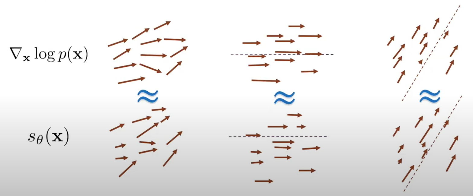
In the image above, the left side shows the goal of matching in all directions, which is not scalable. Instead, we change the problem to match projections along specific directions, indicated by the dotted lines. This approach leads to the following objective:

Sliced Fisher Divergence is the Fisher divergence for projections along random directions, rather than all directions. The formula shows that projection is achieved through inner products:

\[\frac{1}{2} \mathbb{E}_{p_{\mathbf{v}}} \mathbb{E}_{p_{\text {data }}}\left[\left(\mathbf{v}^{\top} \nabla_{\mathbf{x}} \log p_{\theta}(\mathbf{x})-\mathbf{v}^{\top} \nabla_{\mathbf{x}} \log p_{\text {data }}(\mathbf{x})\right)^{2}\right]\]

Using integration by parts, we can rewrite the sliced Fisher divergence as:

\[\mathbb{E}_{p_{\mathbf{v}}} \mathbb{E}_{p_{\text {data }}}\left[\mathbf{v}^{\top} \nabla_{\mathbf{x}}^{2} \log p_{\theta}(\mathbf{x}) \mathbf{v}+\frac{1}{2}\left(\mathbf{v}^{\top} \nabla_{\mathbf{x}} \log p_{\theta}(\mathbf{x})\right)^{2}\right]+\text { const }\]

Sliced score matching offers the advantage of being faster than score matching. Training with this formula results in a finite-sample estimator, making it computable with training data. The random directions \(p_{\mathbf{v}}\) can be sampled from distributions such as the multivariate standard normal or multivariate Rademacher distribution.

This approach significantly reduces computational complexity while maintaining the effectiveness of score matching, making it more practical for high-dimensional data and large-scale applications.

From Score Estimation to Sample Generation

Through score matching, we can now estimate the score from given samples. With the ability to estimate a vector field composed of scores, we can follow the gradient to sample data from high-density regions of the probability distribution. However, simply following the gradient doesn’t guarantee good samples, as we might end up in local optima of the probability distribution.

To overcome this limitation, we can use Langevin dynamics, a type of Markov Chain Monte Carlo (MCMC) method. This approach allows us to explore the distribution without getting trapped in local optima, enabling us to sample from the true underlying distribution.

Langevin Dynamics Sampling

Langevin dynamics sampling follows a specific process. The goal here is to sample from \(p(\mathbf{x})\) using only \(\nabla_{\mathbf{x}} \log p(\mathbf{x})\) (the score function).

The process is as follows:

1. Initialize \(\tilde{\mathbf{x}}_{0} \sim \pi(\mathbf{x})\)
2. Repeat for \(t \leftarrow 1, 2, \cdots, T\): \(\begin{aligned} \mathbf{z}_{t} & \sim \mathcal{N}(0, I) \cr \tilde{\mathbf{x}}_{t} & \leftarrow \tilde{\mathbf{x}}_{t-1}+\frac{\epsilon}{2} \nabla_{\mathbf{x}} \log p\left(\tilde{\mathbf{x}}_{t-1}\right)+\sqrt{\epsilon} \mathbf{z}_{t} \end{aligned}\)

This process differs from simply following the gradient in that it follows a perturbed gradient. Let’s break down the equation:

1. \(\tilde{\mathbf{x}}_{t-1}\) is the current position.
2. \(\frac{\epsilon}{2} \nabla_{\mathbf{x}} \log p\left(\tilde{\mathbf{x}}_{t-1}\right)\) is a step in the direction of the gradient, where \(\epsilon\) is the step size.
3. \(\sqrt{\epsilon} \mathbf{z}_{t}\) is a Gaussian noise term that adds perturbation.

The addition of the Gaussian noise term (the last part of the equation) is crucial. It helps prevent the sampling process from getting stuck in local optima. This noise allows the sampler to explore the entire distribution more effectively, potentially jumping out of local maxima to find the global maximum.

Score-Based Generative Modeling

Based on what we’ve covered so far, we can summarize how score-based generative models create samples.

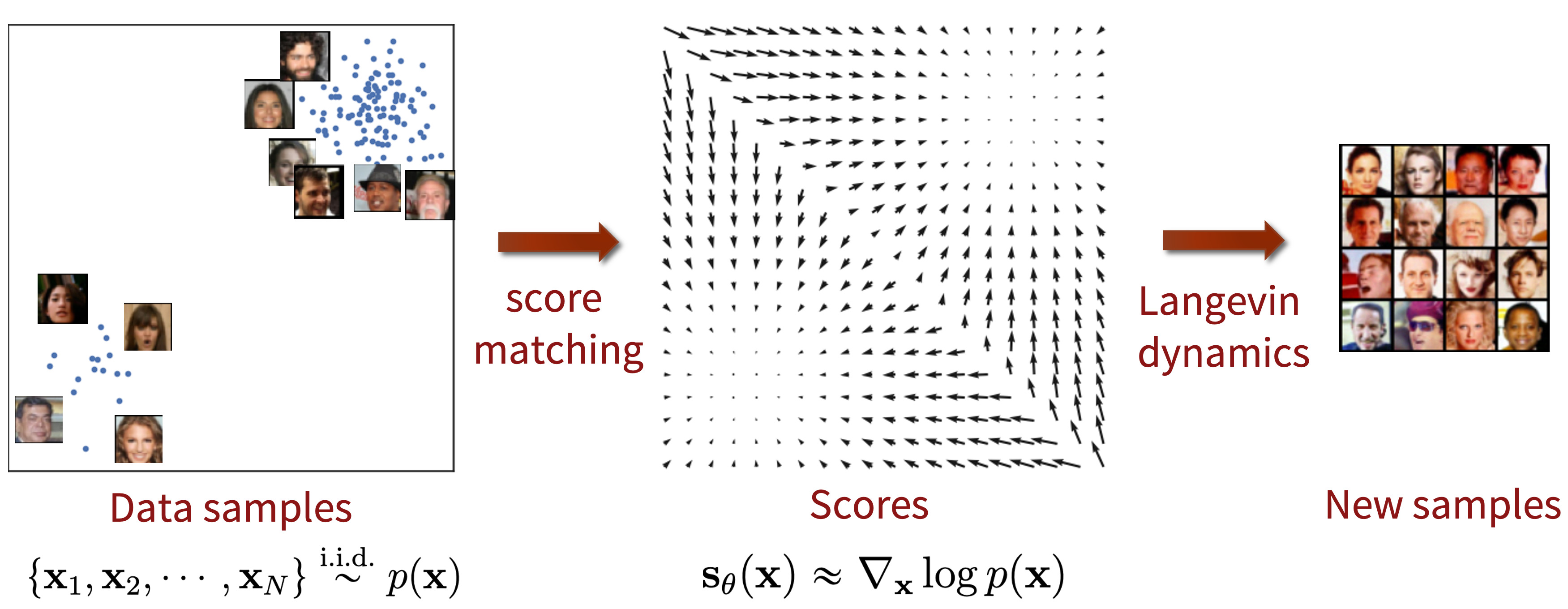
The process of score-based generative modeling can be broken down into three main steps:

1. Construct the training data \(\{\mathbf{x}_1, \mathbf{x}_2, \cdots, \mathbf{x}_{N}\} \stackrel{\text{i.i.d.}}{\sim} p_{\text{data}}(\mathbf{x})\).
2. Use score matching to learn the score function.
3. Generate samples using Langevin dynamics with the learned score function. Since we can now estimate \(\nabla_{\mathbf{x}} \log p_{\text{data}}(\mathbf{x})\) (the gradient of the log-density) using the learned score function, we can employ Langevin dynamics to generate samples.

Pitfalls in Score-Based Generative Models

While the theoretical foundation for score-based generative models is well-established, there are several practical challenges to consider when implementing these models for real-world applications.

Pitfall 1: The Manifold Hypothesis Challenge

The data score is not always well-defined in real-world scenarios. Unlike idealized Gaussian distributions, actual data distributions can be complex and irregular. Consider a ring-shaped data distribution: the score would concentrate around the ring’s edges. If this distribution is narrow, the surrounding gradients would have large values, making it difficult to optimize using gradient-based learning methods.

Pitfall 2: Inaccurate Score Estimation in Low Data-Density Regions

Let’s revisit the gradient plot we discussed earlier:

Naturally, areas with high data density (where many samples exist) allow for more accurate score estimation. However, in regions with low probability density, such as the second and fourth quadrants in this example, the lack of data points leads to highly inaccurate score estimations. This inaccuracy in score estimation ultimately affects the Langevin dynamics process, potentially leading to poor generation results in these areas.

Pitfall 3: Slow Mixing of Langevin Dynamics between Data Modes

Another challenge arises when dealing with mixture distributions. Consider a data distribution composed of two component distributions:

\[p_{\text{data}}(\mathbf{x}) = \pi p_{1}(\mathbf{x}) + (1-\pi) p_{2}(\mathbf{x})\]

Near \(p_{1}\), the estimated score will be close to \(\nabla_{\mathbf{x}} \log p_{1}(\mathbf{x})\), and near \(p_{2}\), it will approximate \(\nabla_{\mathbf{x}} \log p_{2}(\mathbf{x})\). The problem is that when estimating the score, the mixture weight \(\pi\), which plays a crucial role in the actual distribution, is not considered. This can lead to incorrect sampling proportions between different modes of the data distribution, potentially resulting in generated samples that don’t accurately represent the true data distribution.

Gaussian Perturbation

Gaussian perturbation has proven to be an effective approach in addressing the aforementioned issues. The graph below demonstrates how adding a small amount of Gaussian noise to sliced score matching significantly improves the stability of the learning process.

Furthermore, introducing noise allows for more samples to be obtained from low-density regions, thus mitigating the second pitfall. However, it’s important to note that excessive noise can hinder the learning process. Therefore, training with various noise levels has been found to be effective.

This approach, known as annealed Langevin dynamics, involves using a large \(\sigma\) value initially during the Langevin Dynamics sampling process and gradually decreasing \(\sigma\) over time. By employing this annealed method, we can reduce the concentration of sampling around high-density areas, thereby alleviating the previously mentioned pitfalls.

Joint Score Estimation

Even when using annealed Langevin dynamics for sampling, the score estimator needs to be trained on noised samples to predict the correct score. To train on various noise scales, we add isotropic Gaussian noise \(\mathcal{N}(0, \sigma_{i}^{2} I), i=1,2,\cdots,L\) to the samples. The noise levels \(\sigma\) increase as \(i\) approaches \(L\), so \(\sigma_{1} < \sigma_{2} < \cdots < \sigma_{L}\).

The noised distribution is defined as:

\[p_{\sigma_{i}}(\mathbf{x})=\int p(\mathbf{y}) \mathcal{N}\left(\mathbf{x} ; \mathbf{y}, \sigma_{i}^{2} I\right) \mathrm{d} \mathbf{y}\]

To create noised samples, we start with \(\mathbf{x} \sim p(\mathbf{x})\) and add noise \(\mathbf{z} \sim \mathcal{N}(0, I)\) to get \(\mathbf{x} + \sigma_{i} \mathbf{z}\).

To learn the score function for various noise levels, we train a noise-conditional score-based model \(s_{\theta}(\mathbf{x}, i) \approx \nabla_{\mathbf{x}} \log p_{\sigma_{i}}(\mathbf{x})\), where \(\sigma_{i}\) represents different noise levels. This model is conditioned on \(\sigma\), similar to other conditioning models.

In the network architecture, we have \(D\) input dimensions plus an additional input for the noise level \(\sigma\). Thus, \(s_{\theta}(\mathbf{x}, i): \mathbb{R}^{D+1} \rightarrow \mathbb{R}^{D}\). The objective function for \(s_{\theta}(\mathbf{x}, i)\) is defined as a weighted sum of Fisher divergences across noise scales:

\[\sum_{i=1}^{L} \lambda(i) \mathbb{E}_{p_{\sigma_{i}}(\mathbf{x})}\left[ \lVert \nabla_{\mathbf{x}} \log p_{\sigma_{i}}(\mathbf{x})-\mathbf{s}_{\theta}(\mathbf{x}, i) \rVert _{2}^{2}\right]\]

Here, \(\lambda(i) \in \mathbb{R}_{>0}\), and we typically use \(\lambda(i) = \sigma_{i}^2\). The rest of the training process is based on score matching, as explained earlier.

Once we’ve trained the noise-conditional score-based model \(s_{\theta}(\mathbf{x}, i)\), we can generate samples by running Langevin dynamics in the order \(i=L, L-1, \cdots, 1\).

Tuning Score-based Models

The following are recommendations by Yang Song for training score-based generative models with multiple noise scales:

• The noise scales \(\sigma_{1} < \sigma_{2} < \cdots < \sigma_{L}\) should form a geometric sequence. \(\sigma_{1}\) should start from a sufficiently small value, while \(\sigma_{L}\) should be set to approximately the maximum pairwise distance in the dataset. Typically, \(L\) is in the order of hundreds or thousands.
• For the score-based model \(s_{\theta}(\mathbf{x}, i)\), use an architecture with skip connections, such as a U-Net.
• During testing, apply exponential moving average (EMA) to the weights of the score-based model.

Technical details:

1. The geometric sequence of noise scales allows for a smooth transition between different levels of noise, which is crucial for the model to learn a continuous range of data distributions.
2. U-Net architecture with skip connections helps in preserving fine-grained details while also capturing global context, which is particularly useful in image generation tasks.
3. EMA during testing helps stabilize the model’s performance by reducing the impact of short-term fluctuations in the model’s weights during training.

Concluding Remarks

Below are images generated by score-based generative models, demonstrating impressively good results.

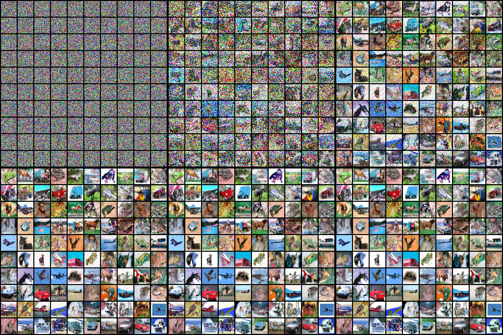
In this article, we explored the underlying theory of score-based generative models. These models represent a new framework in the field of generative modeling, following in the footsteps of GANs, VAEs, and Normalizing Flows. There’s a growing trend of research papers focusing on generative models based on score-based approaches.

As research in this area continues to advance, we can expect to see even more impressive results and potential applications in various domains, from image and video generation to scientific simulations and beyond.

Reference

• Stefano Ermon’s Seminar
• Yang Song’s Blog
• Song, Yang, and Stefano Ermon. “Improved techniques for training score-based generative models.” arXiv preprint arXiv:2006.09011 (2020).